Turning Data into Information Using ArcGIS 10.0 module 5: Identifying a Least Cost Path
Problem: Identifying a least cost path is a common advanced spatial analysis technique and, generally speaking, is considered an optimization problem. Least cost path problems seek to minimize an overall cost associated with a new path between a source and destination point. Cost here can really mean anything, for example taking into account development time or resources required or even more subjective values related to some aesthetic. Some variables may be known or measured and others may be able to be reasonably predicted while some might be subjective. No matter the nature of the variables considered they all must be translated to a common scale so that a cumulative cost can be determined and least cost identified.
The least cost path generated here is for a power transmission line between a power plant site (the fictional Otay Valley Power Plant) and substation (Jamul Substation). The variables to be minimized are monetary cost and public safety cost. Monetary costs are minimized by avoiding steep slope and long paths. Public safety costs are minimized by avoiding residential and commercial zones, open space preserves and public risk areas like airports and lakes.
Analysis Procedures: Ultimately Cost Distance and Cost Direction layers, generated layers that represent 1) how cost varies with distance from the source and 2) local cost obstructions relevant to any particular path, will be combined and analyzed with a Cost Path tool to generate the Least Cost Path. The Cost Distance and Direction layers result from analyzing a Total Cost layers generated by applying a common scaling to the variables of interest. In this case, the variables are slope and land use. A Digital Elevation Model is used to create a Slope layer, whose slopes are then converted to a scale of 1 to 10. Likewise, a Land Use layer is converted to a scale of 1 to 10. In each case 1 translates to least cost and 10 higher cost. The layers can be combined into the Total cost layer after having gone the conversion to a common scale.

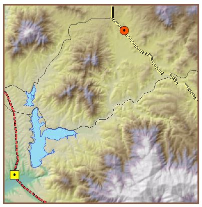
Results: The initial geographic area can be seen here, with the source power plant site as a yellow square and the substation as a red circle. An existing power line is the red dashed line:
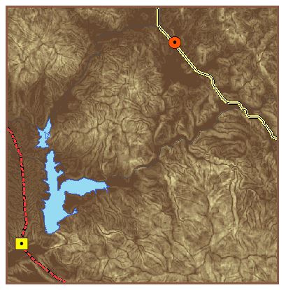
A Slope layer is created from a Digital Elevation Model. The dark brown areas represent low slope areas associated with a lower development cost and the light areas are high cost development areas with a high slope. The brown hues cover a value range from 1 to 10 in preparation for the least cost analysis:
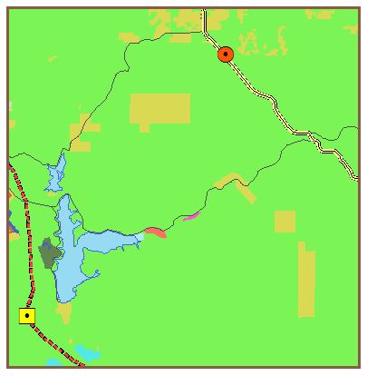
Likewise, Land Use layer is converted to a 1 – 10 scale system so that the layer can be combined with the scaled Slope layer for the cost analysis. Here, land areas that a deemed to have a high development cost associated with them, such as residential or commercial areas, are given a higher value. Land use areas that cannot be considered for the path, such as bodies of water, are given no value so that they are effectively removed from the analysis:
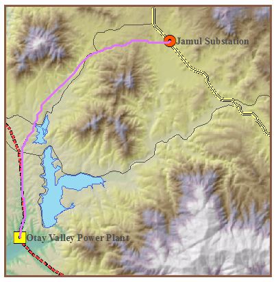
After combining the scaled layers and analyzing with the Path Cost tool an lowest cost path is generated, which is shown here:
Application & Reflection
Problem description: Feasibility assessment to identify a least cost path for a new proposed freeway directly connecting Charlotte and Raleigh.
Data needed: Terrain classification layers, city and county development layers, layers which show restricted land (private holding/preserves/etc).
Analysis procedures: Convert each layer to a 10 point scale indicating suitability for a large scale freeway, including cost associated with terrain types and land tracts that must be avoided. Overlay the results to identify possible (contiguous) lands available for a route.